
Loops of Chaos: Number Patterns in the Lorentz System
📈 Where Numbers Hide in Chaos
In the world of chaos, numbers don’t just tumble out randomly—they spiral, loop, diverge, and return with surprising rhythm. This series explores how classic chaotic systems like Lorentz, Rossler, and Rikitake produce not only beautiful paths in space, but also intricate number streams that hide within them.
In this first post, we’ll dig into the Lorentz system—arguably the most iconic of the chaotic attractors. Instead of focusing on visualizing its 3D trajectory, we’ll inspect what its output looks like when viewed one number at a time.

🔄 A Quick Primer
The Lorentz system is governed by a set of three differential equations. Starting from a chosen point in 3D space (x0, y0, z0), we step forward repeatedly using a numerical integration method. This gives us a stream of (x, y, z) values over time—each one the result of deterministic equations, but seemingly unpredictable if you don’t know the setup.
let x = 0.1, y = 0, z = 0;
const sigma = 10, rho = 28, beta = 8 / 3;
function step() {
const dx = sigma * (y - x);
const dy = x * (rho - z) - y;
const dz = x * y - beta * z;
x += dx * 0.01;
y += dy * 0.01;
z += dz * 0.01;
return { x, y, z };
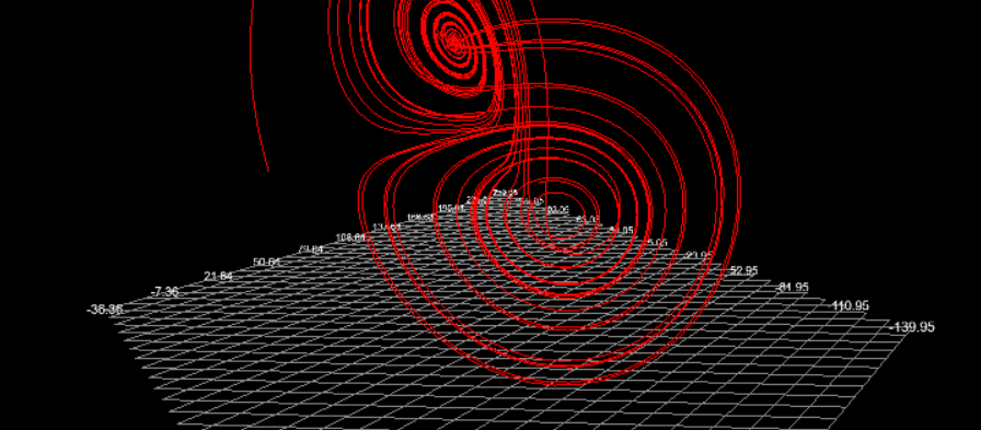
}Each call to step() gives us a new point. Let’s connect these points in 3D and see what we get.
View Image
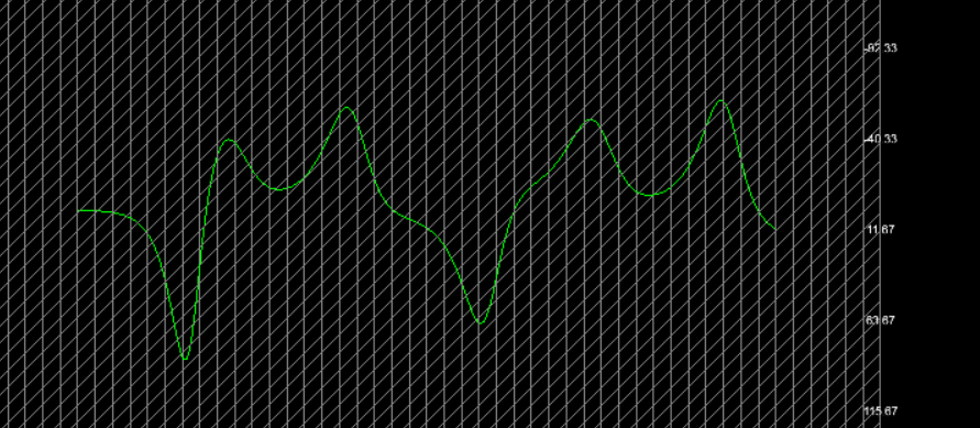
📊 Plotting Chaos One Dimension at a Time
Let’s fix two axes for our plot:
- X-axis: A simple incrementing counter—just the step number.
- Y-axis: The value of one dimension from the Lorentz output (
x,y, orz).
We begin with the vertical component, z. Here’s what it looks like when plotted:
View Image
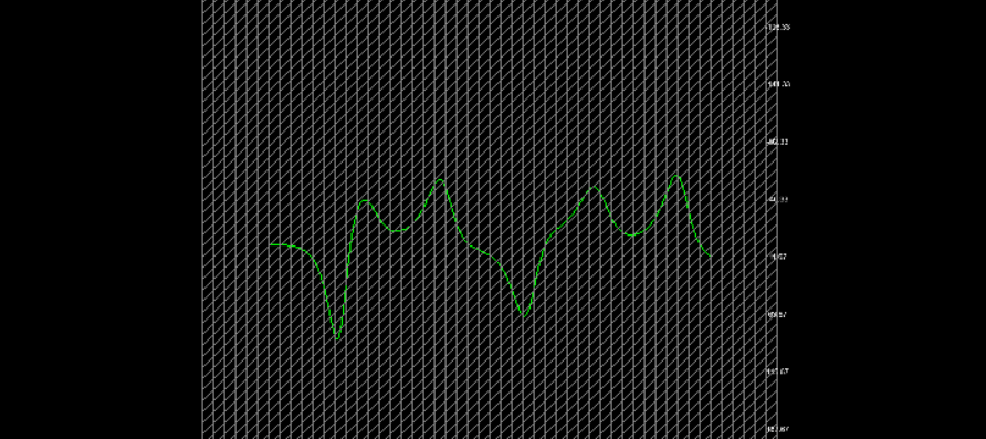
🧮 X, Then Y, Then Both
Next, let’s see the x values.
View Image
Now we plot them together—x and y, step-by-step, using color to separate.
View Image
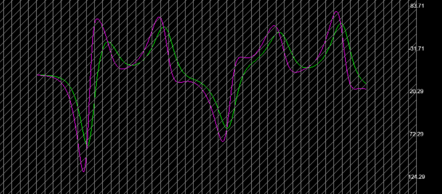
This comparison starts to reveal the interplay between variables. They’re deeply linked, but not in an obvious or linear way. These aren’t just abstract curves—they’re a numeric fingerprint of the chaotic motion of the Lorentz system through space.
This system is defined by these three coupled differential equations:
dx/dt = σ(y - x)
dy/dt = x(ρ - z) - y
dz/dt = xy - βz
🧪 Parameter Tuning and Seed Tweaks
What happens if we:
- Change the step size?
- Alter the starting values?
- Use a slightly different version of the Lorentz equations?
Even small tweaks lead to completely different plots. This is the sensitivity at the heart of chaos theory—a system where small changes have big effects, but still follow rules.
This gives us a powerful tool: controlled randomness. The sequences feel wild, but we can replicate them exactly when needed.
🌀 More Systems, More Shapes
In upcoming posts, we’ll repeat this kind of analysis for other systems:
- Rossler: Smoother, spiral-like behavior
- Rikitake: Loopier, jumpier paths inspired by geomagnetic dynamics
Each system has its own rhythm, and each dimension tells its own story.
📌 Why This Matters
Why look at these numbers at all?
Because they can be:
- Seeds for generative art or procedural animation
- Inputs to systems where repeatable unpredictability is desired
- A window into how structure and randomness coexist in nature
This is about finding patterns where they’re not expected—and learning to listen when systems speak in numbers.
In a later part, we will dive into Rossler’s spiraling patterns and see how a different kind of chaos sings its song.
Let the numbers loop.